Table of Content

• 1. Overview
  • 1.1. Image to Patch Embeddings
  • 1.2. [cls] token and Position Embeddings
  • 1.3. Transformer Encoder
  • 1.4. Image Representation
  • 1.5. Overview with simplified code
• 2. Training
  • 2.1. Fine-Tuning with higher resolution
  • 2.2. Effective with more data
• 3. Experiments
  • 3.1. Comparing to the State of the Art
  • 3.2. Pre-training Data Requirements
  • 3.3. Scaling Study
  • 3.4. Inspecting Vision Transformer
  • 3.5. Attention Map Visualization
• 4. Other experiments and take-aways
  • 4.1. Training and Fine-tuning tricks
  • 4.2. Self-Supervision
  • 4.3. Transformer Shape
  • 4.4. Head Type and [cls] Token
  • 4.5. Positional Embedding
  • 4.6. Empirical Computational Costs
  • 4.7. Axial Attention
• Reference

---

1. Overview

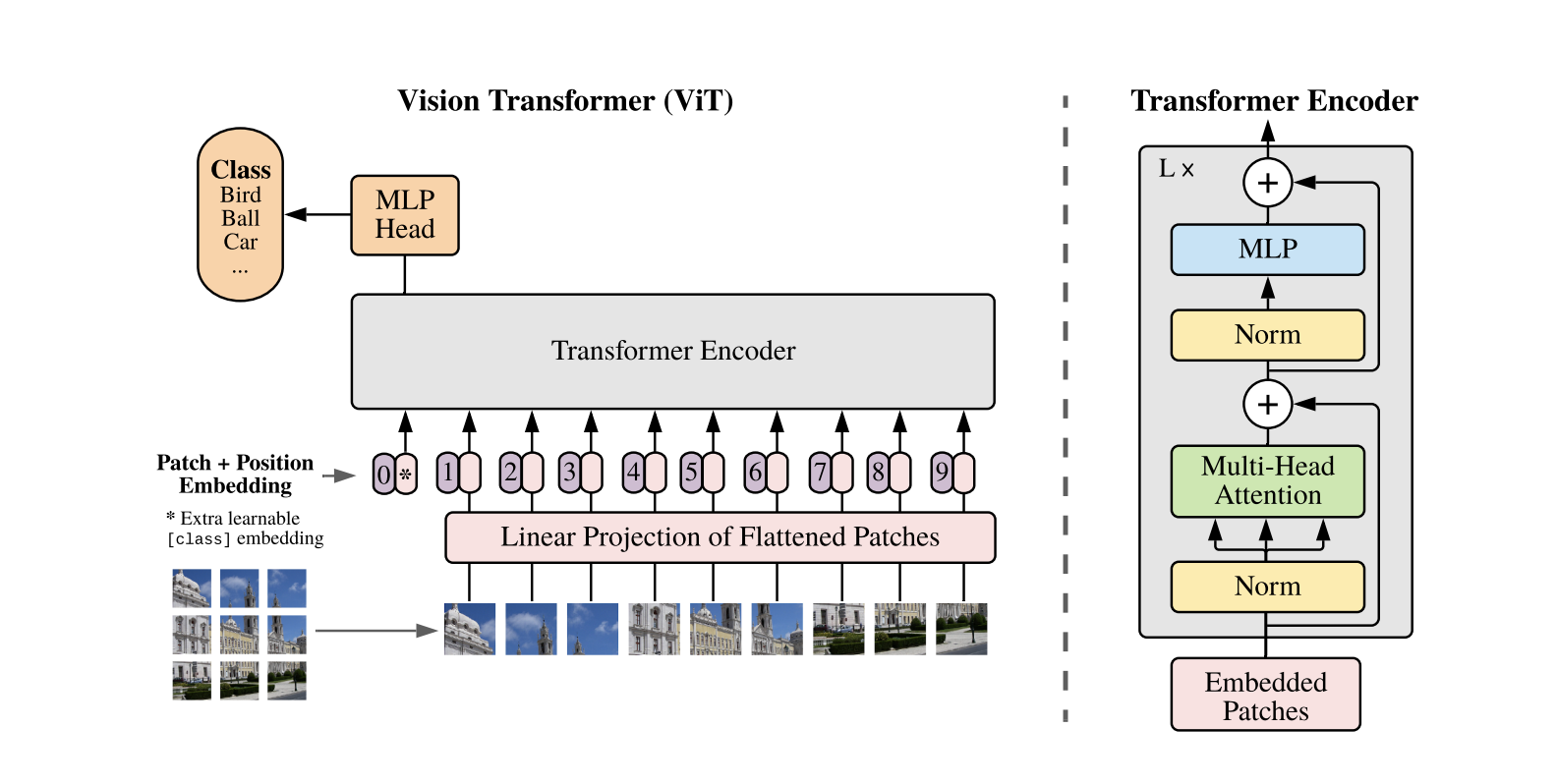
Standard Transformer is applied directly to images, with the fewest possible modification.

1.1. Image to Patch Embeddings

The standard Transformer takes a 1D sequence of token embeddings as input. To handle 2D images, an image is split into $N$ flattened patches ($ x_p^1; x_p^2; \ldots; x_p^N $), each with shape $P^2 \dot C$, where:

• $C$ is the image channels.
• $P^2$ is the patch resolution.
• $N = HW/P^2$ is the patch count and Transformer’s input length, where $HW$ is the image resolution.

These patches are projected to a latent size $D$ as follows:

\[x_p^1 E; x_p^2 E; \ldots; x_p^N E, \quad E \in \mathbb{R}^{(P^2 \cdot C) \times D}\]

As we can see from the simplified code below, patch_embeddings is simply a 2D convolution operation with kernel_size and stride the same as the patch_size. The [cls] token is a vector of the same dimension as the patch tokens.

class Embeddings(nn.Module):
    def forward(self, x):
        # x.shape: [16, 3, 224, 224]
        B = x.shape[0]
        # self.cls_token.shape: [1, 1, 768]
        cls_tokens = self.cls_token.expand(B, -1, -1)
        # cls_tokens.shape: [16, 1, 768]

        # self.patch_embeddings: Conv2d(3, 768, kernel_size=(16, 16), stride=(16, 16))
        x = self.patch_embeddings(x)
        # x.shape: [16, 768, 14, 14]
        x = x.flatten(2)
        # x.shape: [16, 768, 196]
        x = x.transpose(-1, -2)
        # x.shape: [16, 196, 768]
        x = torch.cat((cls_tokens, x), dim=1)
        # x.shape: [16, 197, 768]

        embeddings = x + self.position_embeddings
        # self.position_embeddings.shape: [1, 197, 768]
        embeddings = self.dropout(embeddings)
        return embeddings

1.2. [cls] token and Position Embeddings

A [cls] token is prepend to the sequence. Its state at the output of the Transformer encoder serves as the image representation. Standard learnable 1D position embeddings are added to patch embeddings to retain position information. The position embeddings at initialization time carry no information about the 2D positions of the patches and all spatial relations between the patches have to be learned from scratch.

\[z_0 = \left[ x_{\text{class}}; x_p^1 E; x_p^2 E; \ldots; x_p^N E \right] + E_{\text{pos}}, \quad E \in \mathbb{R}^{(P^2 \cdot C) \times D}, E_{\text{pos}} \in \mathbb{R}^{(N+1) \times D} \quad (1)\]

1.3. Transformer Encoder

The resulting sequence of vectors $z_0$ is fed into a standard Transformer encoder with alternating $MSA$ (multiheaded self-attention) and $MLP$ (multilayer perceptron) blocks. Layer normalization ($LN$) is applied before every block, and residual connections after every block.

\[z'_\ell = \text{MSA}(\text{LN}(z_{\ell-1})) + z_{\ell-1}, \quad (\ell = 1 \ldots L) \quad (2) \\ z_\ell = \text{MLP}(\text{LN}(z'_\ell)) + z'_\ell, \quad (\ell = 1 \ldots L) \quad (3)\]

The encoding process can be depicted as follow:

class Encoder(nn.Module):
    def forward(self, hidden_states):
        # hidden_states.shape: [16, 197, 768]
        # len(self.layer): 12
        for layer_block in self.layer:
            hidden_states, weights = layer_block(hidden_states)
        # self.encoder_norm = LayerNorm(config.hidden_size, eps=1e-6)
        encoded = self.encoder_norm(hidden_states)
        return encoded, attn_weights

For each layer_block in self.layer, the input is passed through a Block module, which contains a $MSA$ module and a $MLP$ module.

class Block(nn.Module):
    def forward(self, x):
        # input: x.shape: [16, 197, 768]

        # MSA: multiheaded self-attention
        h = x
        # self.attention_norm = LayerNorm(config.hidden_size, eps=1e-6)
        x = self.attention_norm(x)
        # self.attn = Attention(config, vis)
        x, weights = self.attn(x)
        x = x + h

        # MLP: multilayer perceptron
        h = x
        # self.ffn_norm = LayerNorm(config.hidden_size, eps=1e-6)
        x = self.ffn_norm(x)
        # self.ffn = Mlp(config)
        x = self.ffn(x)
        x = x + h

        # output: x.shape: [16, 197, 768]
        return x, weights

Details of $MSA$ (multiheaded self-attention):

class Attention(nn.Module):
    def forward(self, hidden_states):
        # hidden_states.shape: [16, 197, 768]

        mixed_query_layer = self.query(hidden_states)
        mixed_key_layer = self.key(hidden_states)
        mixed_value_layer = self.value(hidden_states)
        # shapes: [16, 197, 768]

        query_layer = self.transpose_for_scores(mixed_query_layer)
        key_layer = self.transpose_for_scores(mixed_key_layer)
        value_layer = self.transpose_for_scores(mixed_value_layer)
        # shapes: [16, 12, 197, 64], num_heads = 12

        attention_scores = torch.matmul(query_layer, key_layer.transpose(-1, -2))
        attention_scores = attention_scores / math.sqrt(self.attention_head_size)
        # attention_scores.shape: [16, 12, 197, 197]
        attention_probs = self.softmax(attention_scores)
        weights = attention_probs if self.vis else None
        attention_probs = self.attn_dropout(attention_probs)

        context_layer = torch.matmul(attention_probs, value_layer)
        # context_layer.shape: [16, 12, 197, 64]
        context_layer = context_layer.permute(0, 2, 1, 3).contiguous()
        # context_layer.shape: [16, 197, 12, 64]
        new_context_layer_shape = context_layer.size()[:-2] + (self.all_head_size,)
        context_layer = context_layer.view(*new_context_layer_shape)
        # context_layer.shape: [16, 197, 768]

        # self.out = Linear(config.hidden_size, config.hidden_size)
        attention_output = self.out(context_layer)
        attention_output = self.proj_dropout(attention_output)
        return attention_output, weights

Details of $MLP$ (multilayer perceptron):

class Mlp(nn.Module):
    def forward(self, x):
        # x.shape: [16, 197, 768]
        x = self.fc1(x)
        # x.shape: [16, 197, 3072]

        # self.act_fn = ACT2FN["gelu"]
        x = self.act_fn(x)
        x = self.dropout(x)

        x = self.fc2(x)
        # x.shape: [16, 197, 768]
        x = self.dropout(x)
        return x

1.4. Image Representation

The [cls] token’s state at the output of the Transformer encoder serves as the image representtaion $y$.

\[y = \text{LN}(z_L^0) \quad (4)\]

1.5. Overview with simplified code

The entire process can be also depicted with the following simplified code:

# input.shape: [16, 3, 224, 224], batch_size=16, input_size = 224

embedding_output = Embeddings(x)
# embedding_output.shape: [16, 197, 768], patch_size=16, hidden_size=768
# num_patches = 196 = (224 / 16) ** 2, 197 = 196 + 1

encoded, attn_weights = Encoder(embedding_output)
# encoded.shape: [16, 197, 768]

logits = Head(encoded[:, 0])
# logits.shape: [16, 10], num_classes=10

Both during pre-training and fine-tuning, a classification head (Head) is attached. It is implemented as a $MLP$ with one hidden layer at pre-training time and as a single linear layer at fine-tuning time.

2. Training

2.1. Fine-Tuning with higher resolution

ViT is typically pre-trained on large datasets and fine-tuned for downstream tasks. It’s often beneficial to fine-tune at a higher resolution than the pre-training phase. When feeding images with higher resolution, the patch size stays fixed, therefore increasing the effective sequence length.

Although ViT can handle various sequence lengths, the pre-trained position embeddings may no longer be meaningful. To adjust this, 2D interpolation is applied on the pre-trained position embeddings based on their location in the original image.

This resolution adjustment and patch extraction are the only manually added inductive biases about the image’s 2D structure in ViT.

The following simplified code demonstrates how the position embeddings are adjusted when the grid size is changed from 14 to 21.

# posemb.shape: [1, 197, 768]
posemb_tok, posemb_grid = posemb[:, :0], posemb[0]
# posemb_tok.shape: [1, 1, 768], posemb_grid.shape: [1, 196, 768]
posemb_grid = posemb_grid.reshape(gs_old, gs_old, -1)
# posemb_grid.shape: [14, 14, 768]

# gs_old = 14, gs_new = 21
zoom = (gs_new / gs_old, gs_new / gs_old, 1)
# zoom = (1.5, 1.5, 1)
# The array is zoomed using spline interpolation of the requested order.
posemb_grid = ndimage.zoom(posemb_grid, zoom, order=1)
posemb_grid = posemb_grid.reshape(1, gs_new * gs_new, -1)
# posemb_grid.shape: [1, 441, 768]

posemb = np.concatenate([posemb_tok, posemb_grid], axis=1)
# posemb.shape: [1, 442, 768]

2.2. Effective with more data

When trained on mid-sized datasets like ImageNet without strong regularization, ViT underperforms similar-sized ResNets. Because Transformers lack certain inductive biases inherent to CNNs, such as translation equivariance and locality, which affects their performance with limited data.

However, when trained on larger datasets (14M-300M images), ViT approaches or beats state-of-the-art results in various image recognition benchmarks. It seems that large scale training trumps inductive bias.

3. Experiments

3.1. Comparing to the State of the Art

Vision Transformer models pre-trained on the JFT-300M dataset outperform ResNet-based baselines on all datasets, while taking substantially less computational resources to pre-train. ViT pre-trained on the smaller public ImageNet-21k dataset performs well too.

^{Image source: original paper Table 2}

The ViT-L/16 model pre-trained on the public ImageNet-21k dataset performs well on most datasets too, while taking fewer resources to pre-train: it can be trained on an 8-core cloud TPUv3 in roughly 30 days (0.23k / 8 = 28.75).

The figure below decomposes the VTAB tasks into their respective groups, and compares ViT with previous SOTA methods on this benchmark: BiT, VIVI – a ResNet co-trained on ImageNet and Youtube, and S4L – supervised plus semi-supervised learning on ImageNet.

^{Image source: original paper Figure 2}

ViT-H/14 outperforms BiT-R152x4, and other methods, on the Natural and Structured tasks. On the Specialized the performance of the top two models is similar.

3.2. Pre-training Data Requirements

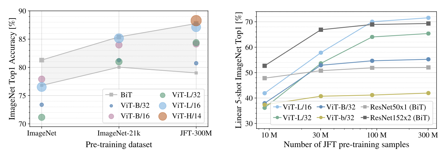^{Image source: original paper Figure 3 & 4}

• (Left): While ViT models underperform BiT ResNets (shaded area) when pre-trained on small datasets, they excel when pre-trained on larger datasets. Similarly, larger ViT variants overtake smaller ones as the dataset grows.
• (Right): The models are trained on subsets of 9M, 30M, 90M, and the complete JFT-300M dataset. To save compute, few-shot linear accuracy instead of full finetuning accuracy is reported. While ResNets perform better with smaller pre-training datasets, they plateau sooner than ViT, which performs better with larger pre-training.

3.3. Scaling Study

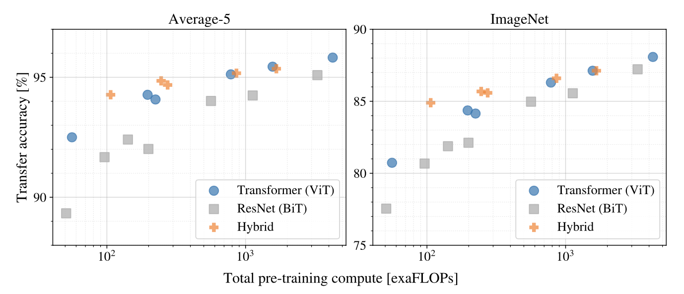^{Image source: original paper Figure 5}

• Vision Transformers generally outperform ResNets in terms of performance-to-compute efficiency. On average across five datasets, ViT achieves comparable performance with 2 to 4 times less compute.
• While hybrids have a slight edge over ViT with limited computational resources, this advantage fades with larger models. This is unexpected, as one might anticipate the benefits of convolutional local features to persist irrespective of ViT’s size.
• There’s no evident performance saturation for Vision Transformers within the experimented range, suggesting potential in further scaling efforts.

The hybrid architecture

As an alternative to raw image patches, the input sequence can be formed from feature maps of a CNN, and the patch embedding projection $E$ is applied to patches extracted from a CNN feature map.

As a special case, the patches can have spatial size 1x1, which means that the input sequence is obtained by simply flattening the spatial dimensions of the feature map and projecting to the Transformer dimension.

3.4. Inspecting Vision Transformer

^{Image source: original paper Figure 7}

• (Left): The top principal components of the learned embedding filters of the first layer of the Vision Transformer. The components resemble plausible basis functions for a low-dimensional representation of the fine structure within each patch.
• (Center): The model encodes intra-image distances through position embeddings, meaning nearer patches often have analogous embeddings. Additionally, the row-column structure is evident as patches in the same row/column share similar embeddings.
• (Right): Size of attended area by head and network depth. Some heads attend to most of the image already in the lowest layers, showing that the ability to integrate information globally is indeed used by the model. Other attention heads have consistently small attention distances in the low layers. The attention distance increases with network depth.

3.5. Attention Map Visualization

Globally, the model seems to attend to image regions that are semantically relevant for classification.

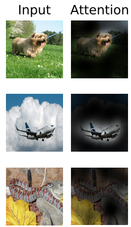^{Image source: original paper Figure 6}

Attention Rollout is used to compute maps of the attention from the output token to the input space.

Attention Rollout

According to this notebook, attention rollout is implemented as follow:

Step 1: Extract attention weights for each layer

x = transform(im)
logits, att_mat = model(x.unsqueeze(0))

In the above code, att_mat is a list of weights, each is shaped [1, 12, 197, 197]. The weights is just the attention_probs from the attention layer (12 heads).

Step 2: Aggregate and normalize the attention weights

Combine the attention weights from all heads and average them.

att_mat = torch.stack(att_mat).squeeze(1)
# att_mat.shape: [12, 12, 197, 197], 12 heads, 12 layers
att_mat = torch.mean(att_mat, dim=1)
# att_mat.shape: [12, 197, 197], average across heads

To account for residual connections, add an identity matrix to the attention matrix and normalize the result.

residual_att = torch.eye(att_mat.size(1))
aug_att_mat = att_mat + residual_att
aug_att_mat = aug_att_mat / aug_att_mat.sum(dim=-1).unsqueeze(-1)

Step 3: Compute the cumulative attention map across layers

The aggregated attention map for all layers can be derived by recursively multiplying weight matrices.

joint_attentions = torch.zeros(aug_att_mat.size())
joint_attentions[0] = aug_att_mat[0]

for n in range(1, aug_att_mat.size(0)):
    joint_attentions[n] = torch.matmul(aug_att_mat[n], joint_attentions[n-1])

Step 4: Visualize the attention map

We only focus on the attention from the [cls] token to the original image’s positions.

v = joint_attentions[-1]
# v.shape: [197, 197]
grid_size = int(np.sqrt(aug_att_mat.size(-1)))
mask = v[0, 1:].reshape(grid_size, grid_size).detach().numpy()
# mask.shape: [14, 14]
mask = cv2.resize(mask / mask.max(), im.size)[..., np.newaxis]
result = (mask * im).astype("uint8")

In the end, the visualization is displayed:

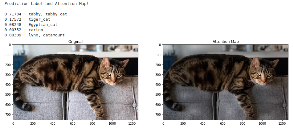
We can also visualize the attention map of individual layers, simply iterate through joint_attentions.

4. Other experiments and take-aways

4.1. Training and Fine-tuning tricks

• Strong regularization is the key when training models from scratch on ImageNet.
• Using Adam as the optimizer for pre-training ResNets on JFT has been found to be more effective, although ResNets are usually trained with SGD.
• ViT models are fine-tuned using SGD, utilizing a momentum of 0.9. Learning rates are determined by grid searching, with subsets of the training data serving as a development set. The full training set is used for final training.
• It’s standard to use different resolutions for training and fine-tuning. For example, ViT-B/16 is pre-trained on 224x224 images and fine-tuned on 384x384 images.
• When adapting ViT models for new datasets, the entire head, which consists of two linear layers, is replaced with a single zero-initialized linear layer to match the class count of the target dataset. This approach proves more stable than merely re-initializing the final layer.

4.2. Self-Supervision

4.2.1. Objective

The primary task is masked patch prediction. Just like a jigsaw puzzle, where some pieces (or patches) of the image are hidden, and the model’s job is to predict information about these hidden patches.

50% of the patches in an image are “corrupted” in one of three ways:

• 80% of the time, the embeddings of these patches are replaced with a learnable [mask] embedding.
• 10% of the time, they are replaced with the embedding of a random different patch.
• The remaining 10% of the time, the patches are left unchanged.

4.2.2. Prediction Targets

These are the things that the model tries to predict for each corrupted patch:

• Mean 3-bit Color: predict an approximate average color for each hidden patch.
  • The model tries to predict the average color of the corrupted patch.
  • This average color is quantized into 3 bits, so there are 512 possible colors the model can predict (2^3 for each RGB channel).
• Downsampled Version: a bit more detailed than the first option, as the model tries to capture more localized color information within the patch.
  • Instead of predicting just one average color, the model predicts colors for a 4x4 downsized version of the original 16x16 patch.
  • Each of these 16 smaller sections in the downsized version has its color predicted, just like in the first setting. This results in the model making 16 predictions, each of which can be one of the 512 possible colors.
• Regression on the Full Patch: With a 16x16 patch, this leads to 256 predictions (one for each pixel), where each prediction is a set of RGB values.
  • Here, the model tries to predict the actual RGB values of all the pixels in the corrupted patch.
  • This is a regression task because the model is trying to predict continuous values (RGB values) rather than picking from a predefined set.

4.2.3. Results

• All three methods seemed to work decently. However, the L2 regression approach was a bit worse than the other two. The first method (predicting the mean 3-bit color) is selected finally because it gave the best performance in few-shot learning scenarios.
• It’s found that corrupting only 15% of the patches, as used in a previous study, was less effective than corrupting 50%.
• This approach didn’t need extensive pretraining or massive datasets to achieve good performance on ImageNet classification.
• Diminishing benefits appear after 100k pretraining steps and noted that pretraining just on ImageNet yielded comparable gains.

4.3. Transformer Shape

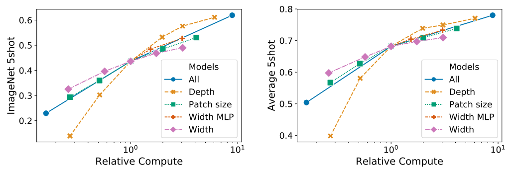^{Image source: original paper Figure 8}

Scaling network width has minimal impact. Reducing patch size, which increases sequence length, notably improves performance without adding parameters. This indicates compute might better predict performance than parameter count, and depth should be prioritized over width. Proportional scaling across all dimensions enhances results.

4.4. Head Type and [cls] Token

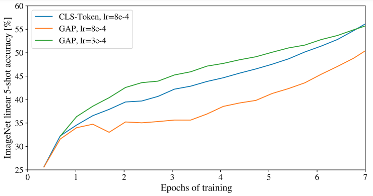^{Image source: original paper Figure 9}

Apart from using the [cls] token as in the standard Transformer, we can just apply global average-pooling (GAP) on the image-patch embeddings, and then use a linear classifier, just like ResNet’s final feature. This approach performs comparably to the [cls] token but necessitates different learning rates.

4.5. Positional Embedding

Different ways of incorporating spatial information via positional embedding are investigated:

• No positional info: Treating inputs as an unordered collection of patches.
• 1D positional embedding: Sequencing patches in raster order (from left to right, top to bottom, similar to reading English text).
• 2D positional embedding: Structuring patches in a 2D grid, using X and Y embeddings, combined for each patch’s final position.
• Relative positional embeddings: Using relative distances between patches instead of fixed positions, leveraging 1D Relative Attention.

Additionally, for 1D and 2D embeddings, three integration approaches were tested:

• Adding positional embeddings to the model’s stem before the Transformer (default).
• Adding unique positional embeddings at the start of each layer.
• Layer-shared positional embeddings added at each layer’s start.

^{Image source: original paper Table 8}

The results indicate while positional embeddings significantly outperform no embeddings, the specific embedding type made minor differences. This could be due to Transformer working on patch-level inputs with reduced spatial dimensions, making different encoding strategies equally effective.

4.6. Empirical Computational Costs

The inference speed of key models is tested on a TPUv3 accelerator.

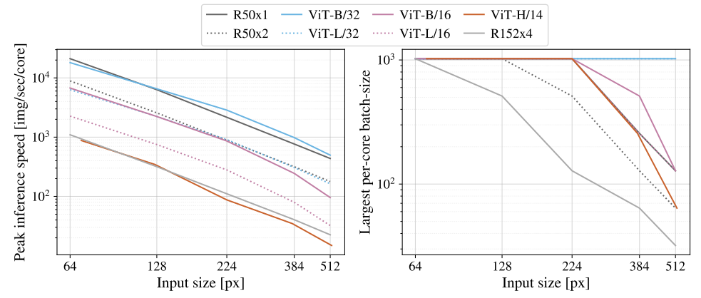^{Image source: original paper Figure 12}

• (Left): How many images one core can handle per second, across various input sizes. ViT models have speed comparable to similar ResNets.
• (Right): The largest batch-size each model can fit onto a core, larger being better for scaling to large datasets. ViT models are clearly more memory-efficient.

4.7. Axial Attention

Axial Attention efficiently handles large multidimensional tensor inputs by applying attention operations along individual tensor axes, rather than flattening them. This approach is employed in the AxialResNet baseline.

The ViT model was modified to handle 2D-shaped inputs and was incorporated with Axial Transformer blocks. The typical self-attention and MLP combination is replaced by row self-attention with an MLP, followed by column self-attention with an MLP.

Axial-ViT models outperform the standard ViT-B versions but require more computational resources. In Axial-ViT, each global self-attention Transformer block is swapped for two Axial ones, and even though they operate on shorter sequences, there’s an added MLP in each block.

AxialResNet’s performance appears efficient in terms of accuracy vs. compute trade-off, but it’s notably slow on TPUs.

Reference

• Paper: An Image is Worth 16x16 Words: Transformers for Image Recognition at Scale
• Code: https://github.com/jeonsworld/ViT-pytorch