Table of Content
- 1. Approach
- 2. Architecture
- 3. Training
- 4. Experiments
- 5. Comparison to Human Performance
- 6. Data Overlap Analysis
- 7. Limitations
- Afterwords: Thoughts on CLIP
- Reference
Launched in early 2021, CLIP (Contrastive Language–Image Pre-training) has sparked numerous creative projects. Its influence in inspiring diverse innovations is noteworthy. Exploring the original paper and its code is highly recommended.
This article provides an annotated version of the CLIP paper, examining implementation details using the open-source implementation of CLIP. We also demonstrate the training process using a small dataset. Where the paper’s content doesn’t directly relate to code, we summarize key concepts, adding insights and comments.
Reading papers in this way deepens my understanding, and I hope it is helpful for you as well.
1. Approach
1.1. Benefits of Natural Language Supervision
Scaling up natural language supervision is straightforward because it can learn passively from the extensive amount of text available on the internet.
Moreover, it not only acquires a visual representation but also establishes connections between that representation and language, facilitating flexible zero-shot transfer.
1.2. Create a Sufficiently Large, Diverse, and Balanced Dataset
A major motivation for natural language supervision is the vast amount of this type of data available publicly on the internet. However, no existing dataset is large enough to fully capture this potential.
Therefore, the authors constructed a new dataset comprising 400 million (image, text) pairs, collected from a variety of publicly available sources on the internet. This dataset is referred to as WIT, standing for WebImageText.
In the process of creating this dataset, the goal was to cover as broad a range of visual concepts as possible, utilizing a set of 500,000 queries. To maintain class balance, up to 20,000 (image, text) pairs per query were included.
1.3. Select an Efficient Pre-Training Method to Enable Scalable Training
Efficient training was crucial for scaling up natural language supervision due to the extensive model and dataset sizes.
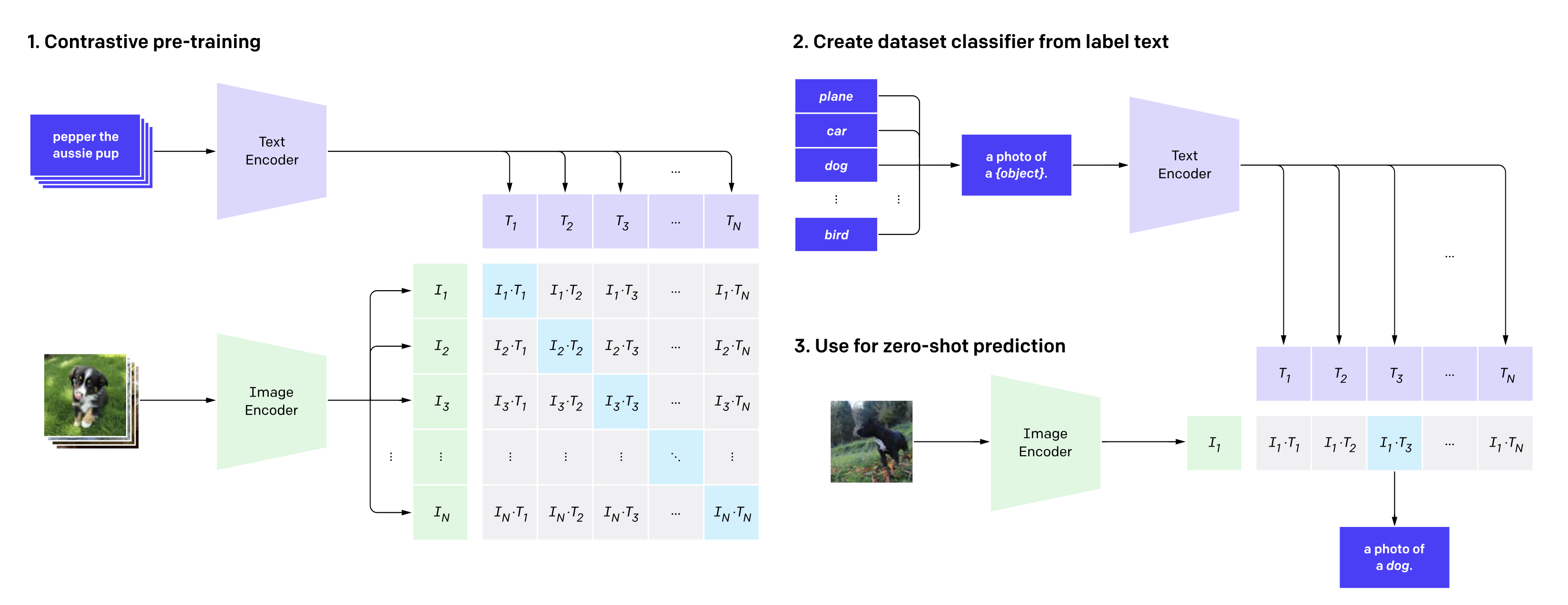
The initial attempt was made to train an image CNN and text transformer from scratch to predict image captions; however, this method was inefficient. The complexity of the task was amplified by the fact that images can correspond to a multitude of texts. A more streamlined approach was selected: training the model to associate texts with their corresponding images from a batch of N (image, text) pairs.
To achieve this, CLIP learns a multi-modal embedding space where image and text encoders are trained to enhance the cosine similarity between the image and text embeddings of the N pairs that are paired in the training set, while diminishing it for other pairings, which are not inherently incorrect but simply do not appear together in the training set.
2. Architecture
2.1. Image Encoder
Two different architectures have been considered for the image encoder.
2.1.1. Modified ResNet
For the first, ResNet-50 is used as the base architecture for the image encoder due to its widespread adoption and proven performance. Comparing to the original architecture, Modified ResNet undergoes several modifications:
-
Instead of a single “stem” convolution, there are three. Additionally, an average pool replaces the max pool.
-
Normal ResNet:
# x: [n, 3, 224, 224] -> [n, 64, 56, 56] # stem self.conv1 = nn.Conv2d(3, self.inplanes, kernel_size=7, stride=2, padding=3, bias=False) self.bn1 = norm_layer(self.inplanes) self.relu = nn.ReLU(inplace=True) self.maxpool = nn.MaxPool2d(kernel_size=3, stride=2, padding=1) -
Modified ResNet:
# x: [n, 3, 224, 224] -> [n, 64, 56, 56]
# stem1
self.conv1 = nn.Conv2d(3, width // 2, kernel_size=3, stride=2, padding=1, bias=False)
self.bn1 = nn.BatchNorm2d(width // 2)
self.act1 = nn.ReLU(inplace=True)

# stem2
self.conv2 = nn.Conv2d(width // 2, width // 2, kernel_size=3, padding=1, bias=False)
self.bn2 = nn.BatchNorm2d(width // 2)
self.act2 = nn.ReLU(inplace=True)

# stem3
self.conv3 = nn.Conv2d(width // 2, width, kernel_size=3, padding=1, bias=False)
self.bn3 = nn.BatchNorm2d(width)
self.act3 = nn.ReLU(inplace=True)

self.avgpool = nn.AvgPool2d(2)
-
-
It performs anti-aliasing strided convolutions within the
Bottleneckblock, where anavgpoolis prepended to convolutions withstride > 1. The idea is that, when the stride is greater than 1, instead of just doing a strided convolution (which can cause aliasing), the model would perform average pooling before the convolution. This can reduce the aliasing effect.-
Normal ResNet:
if stride != 1 or self.inplanes != planes * block.expansion: downsample = nn.Sequential( conv1x1(self.inplanes, planes * block.expansion, stride), norm_layer(planes * block.expansion), ) -
Modified ResNet:
if stride > 1 or inplanes != planes * Bottleneck.expansion:
    self.downsample = nn.Sequential(
        OrderedDict(
            [
                ("-1", nn.AvgPool2d(stride)),
                (
                    "0",
                    nn.Conv2d(
                        inplanes, planes * self.expansion, 1, stride=1, bias=False
                    ),
                ),
                ("1", nn.BatchNorm2d(planes * self.expansion)),
            ]
        )
    )
-
-
The final pooling layer is a
QKVattention instead of an average pool.
2.1.2. Vision Transformer (ViT)
For the second, the recently introduced Vision Transformer (ViT) is examined. The implementation closely mirrors the original, with the minor modification of adding an extra layer normalization to the combined patch and position embeddings before the transformer, and a slightly different initialization scheme is utilized.
Here ViT-B/16 is used to showcase the forward process.
class VisionTransformer(nn.Module):
    def forward(self, x: torch.Tensor):
        # x.shape: [8, 3, 224, 224]
        x = self.conv1(x)
        # x.shape: [8, 768, 14, 14], 224 / 16 = 14
        x = x.reshape(x.shape[0], x.shape[1], -1)
        # x.shape: [8, 768, 196]
        x = x.permute(0, 2, 1)
        # x.shape: [8, 196, 768]

        # class embeddings
        # self.class_embedding.shape: [768]
        # [768] + [8, 1, 768] -> [8, 1, 768]
        x = torch.cat(
            [
                self.class_embedding.to(x.dtype)
                + torch.zeros(
                    x.shape[0], 1, x.shape[-1], dtype=x.dtype, device=x.device
                ),
                x,
            ],
            dim=1,
        )

        # positional embeddings
        # x.shape: [8, 197, 768]
        # self.positional_embedding.shape: [197, 768]
        x = x + self.positional_embedding.to(x.dtype)

        x = self.patch_dropout(x)
        # the minor modification
        x = self.ln_pre(x)

        # x.shape: [8, 197, 768]
        x = x.permute(1, 0, 2)
        # x.shape: [197, 8, 768]
        x = self.transformer(x)
        # x.shape: [197, 8, 768]
        x = x.permute(1, 0, 2)
        # x.shape: [8, 197, 768]

        # self._global_pool simply returns x[:, 0], x[:, 1:]
        pooled, tokens = self._global_pool(x)
        # pooled.shape: [8, 768], tokens.shape: [8, 196, 768]
        pooled = self.ln_post(pooled)

        if self.proj is not None:
            # self.proj.shape: [768, 512]
            pooled = pooled @ self.proj
            # pooled.shape: [8, 512]

        if self.output_tokens:
            return pooled, tokens

        return pooled
Specifically, self.transformer is a Transformer object:
class Transformer(nn.Module):
    def forward(self, x: torch.Tensor, attn_mask: Optional[torch.Tensor] = None):
        # 12 * ResidualAttentionBlock
        # x.shape: [197, 8, 768]
        for r in self.resblocks:
            if self.grad_checkpointing and not torch.jit.is_scripting():
                # ...
            else:
                x = r(x, attn_mask=attn_mask)

        # x.shape: [197, 8, 768]
        return x

class ResidualAttentionBlock(nn.Module):
    def forward(
        self,
        q_x: torch.Tensor,
        k_x: Optional[torch.Tensor] = None,
        v_x: Optional[torch.Tensor] = None,
        attn_mask: Optional[torch.Tensor] = None,
    ):
        # q_x.shape: [197, 8, 768]
        k_x = (
            self.ln_1_kv(k_x) if hasattr(self, "ln_1_kv") and k_x is not None else None
        )
        v_x = (
            self.ln_1_kv(v_x) if hasattr(self, "ln_1_kv") and v_x is not None else None
        )
        # k_x, v_x both are None

        # self.attention: MultiheadAttention, n_head = 12
        x = q_x + self.ls_1(
            self.attention(q_x=self.ln_1(q_x), k_x=k_x, v_x=v_x, attn_mask=attn_mask)
        )
        # x.shape: [197, 8, 768]

        # self.mlp
        # Sequential(
        #   (c_fc): Linear(in_features=768, out_features=3072, bias=True)
        #   (gelu): GELU(approximate='none')
        #   (c_proj): Linear(in_features=3072, out_features=768, bias=True)
        # )
        x = x + self.ls_2(self.mlp(self.ln_2(x)))

        return x
2.2. Text encoder
The text encoder is a modified Transformer model with 63M parameters, featuring 12 layers, a width of 512, and 8 attention heads. It processes text using lower-cased byte pair encoding (BPE) with a 49,152 vocab size, and limits the max sequence length to 76 for efficiency.
Text sequences begin and end with [SOS] (start of sentence) and [EOS] (end of sentence) tokens. The text’s feature representation is obtained from the [EOS] token activations in the transformer’s top layer. These activations undergo layer normalization and linear projection into a multi-modal embedding space.
The feed-forward encoding process:
class CLIP(nn.Module):
    def encode_text(self, text, normalize: bool = False):
        cast_dtype = self.transformer.get_cast_dtype()
        # text[0]: [49406,   320,  1876,  8192,  1417,   518,  1573,   269, 49407]
        x = self.token_embedding(text).to(cast_dtype)
        # [batch_size, 77, 512]
        x = x + self.positional_embedding.to(cast_dtype)
        x = x.permute(1, 0, 2)
        # [77, batch_size, 512]

        x = self.transformer(x, attn_mask=self.attn_mask)
        # [77, batch_size, 512]

        x = x.permute(1, 0, 2)
        # [77, batch_size, 512]
        x = self.ln_final(x)
        x = x[torch.arange(x.shape[0]), text.argmax(dim=-1)] @ self.text_projection
        # [batch_size, 1024]
        return F.normalize(x, dim=-1) if normalize else x
3. Training
3.1. Model Scaling: Allocate Additional Compute across Width, Depth, and Resolution
Previous computer vision research typically scaled models by increasing either width or depth. In contrast, this approach distributes additional compute across width, depth, and resolution in ResNet image encoders.
For the text encoder, scaling is limited to the model’s width, matching the proportional increase in the ResNet’s width, since CLIP’s performance was found to be less sensitive to the capacity of the text encoder.
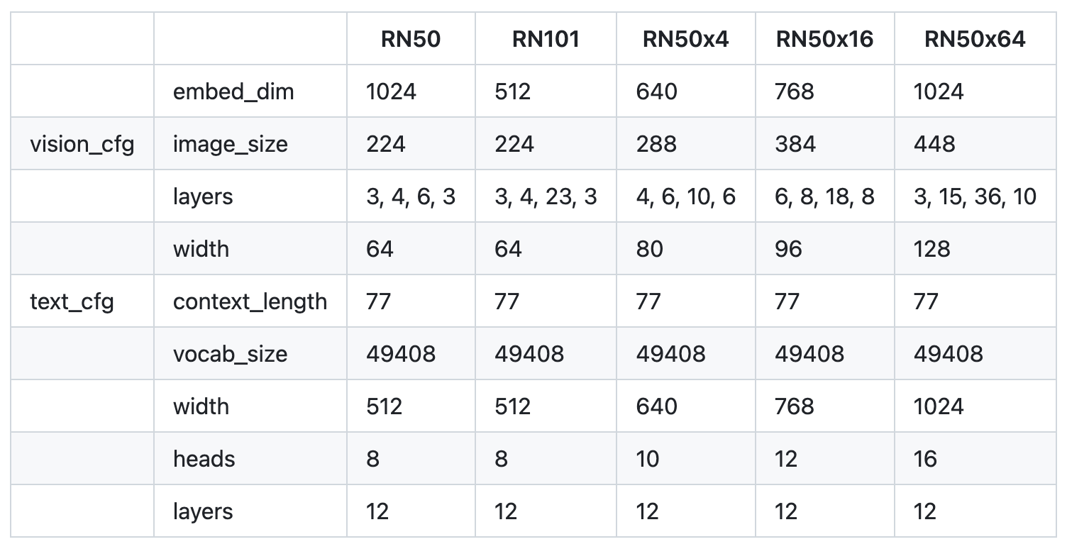 A series of 5 ResNets and the corresponding text encoders.
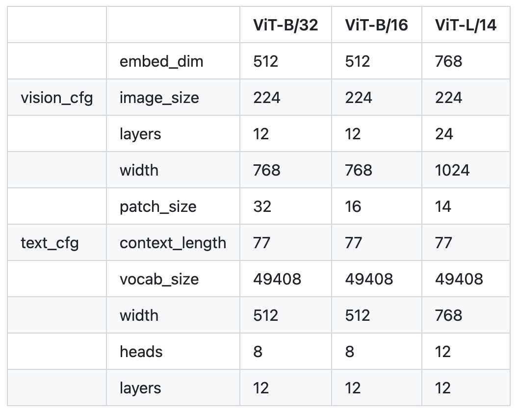 A series of 3 Vision Transformers and the corresponding text encoders.
Reference: open_clip/model_configs
All models undergo 32 epochs of training with a large minibatch size of 32,768.
The largest ResNet model, RN50x64, takes 18 days to train on 592 V100 GPUs. In comparison, the biggest Vision Transformer finishes training in 12 days on 256 V100 GPUs, making it the preferred image encoder due to its efficiency.
Additionally, the ViT-L/14 undergoes an extra epoch of pre-training at 336 pixels resolution, known as ViT-L/14@336px. This version is primarily referenced as “CLIP” in the paper, identified as the most effective model.
3.2. Training: Bag of Tricks to Improve Efficiency and Stability
3.2.1. Adam optimizer with decoupled weight decay regularization
optimizer = optim.AdamW(
    [
        {"params": gain_or_bias_params, "weight_decay": 0.0},
        {"params": rest_params, "weight_decay": args.wd},
    ],
    lr=args.lr,
    betas=(args.beta1, args.beta2),
    eps=args.eps,
)
Weight decay regularization is applied to all weights except gains and biases.
Gains, key to stabilization in normalization layers ("bn", "ln", "logit_scale"), maintain activation stability. Applying weight decay to these can upset this balance, causing the network to compensate by adjusting preceding layer weights, which may lead to instability.
Biases are essential for shifting activations and fitting data. Weight decay on biases might restrict network capacity, especially in deep networks or those with saturating activation functions. With biases comprising fewer parameters than weights, their regularization has a minimal role in preventing overfitting. Free adjustment of biases improves data fitting and model performance.
3.2.2. Cosine learning rate schedule with linear warmup
The intuition behind is to start with a higher learning rate to help the model quickly find a region of the parameter space close to the optimal solution, and then gradually decrease the learning rate to refine the solution. It also combine the benefits of a warm-up phase for stabilizing the initial training period.
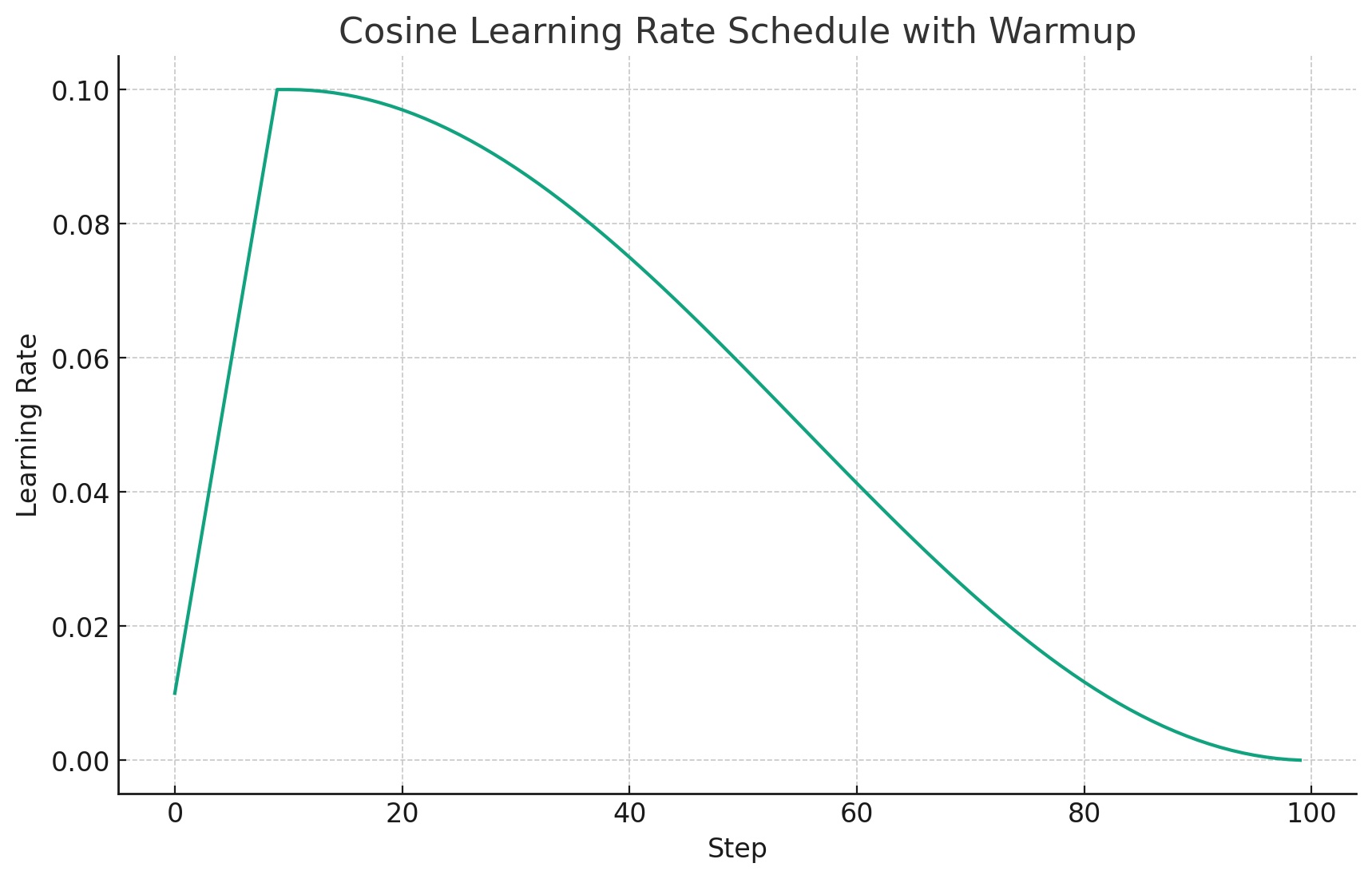
def cosine_lr(base_lr, warmup_length, steps):
    lrs = []
    for step in range(steps):
        if step < warmup_length:
            lr = _warmup_lr(base_lr, warmup_length, step)
        else:
            e = step - warmup_length
            es = steps - warmup_length
            lr = 0.5 * (1 + np.cos(np.pi * e / es)) * base_lr
        lrs.append(lr)
    return lrs

def _warmup_lr(base_lr, warmup_length, step):
    return base_lr * (step + 1) / warmup_length
3.2.3. Gradient checkpointing
class Transformer(nn.Module):
    def forward(self, x: torch.Tensor, attn_mask: Optional[torch.Tensor] = None):
        for r in self.resblocks:
            if self.grad_checkpointing and not torch.jit.is_scripting():
                x = checkpoint(r, x, None, None, attn_mask)
            else:
                x = r(x, attn_mask=attn_mask)
        return x
Gradient checkpointing is a technique used during the training of deep neural networks to reduce the memory consumption of the backward pass (i.e., when computing gradients for backpropagation). It trades off computation time for memory space. This technique is particularly useful for training very deep networks that otherwise wouldn’t fit into memory.
The basic idea behind backpropagation in neural networks is to compute the gradient of the loss with respect to the network’s parameters. To do this, during the forward pass, intermediate activations for each layer are stored in memory. During the backward pass, these stored activations are used to compute the gradients layer-by-layer. In very deep networks, storing all these intermediate activations can be memory-intensive. This is where gradient checkpointing comes in.
Here’s how gradient checkpointing works:
- Decompose the Network: Instead of storing the intermediate activations for every layer, you store them for only a subset of layers. These stored layers act as “checkpoints.”
- Recompute Activations: During the backward pass, when you need an activation that was not stored, you recompute it. Starting from the nearest checkpoint, you perform a mini forward pass to get the required activation.
- Backward Pass as Usual: Once you have the required activation, you can proceed with the backward pass as usual.
Example:
- Consider a deep network with 100 layers. Without gradient checkpointing, during training, you’d store the activations for every layer from 1 to 100.
- With gradient checkpointing, you might store activations only for layers 1, 20, 60, 80.
- If you need the activations for layer 30 during the backward pass, you’d recompute it starting from layer 20.
Benefits:
- Memory Savings: By not storing every intermediate activation, you save a significant amount of memory.
Drawbacks:
- Increased Computation: Since some activations are recomputed during the backward pass, gradient checkpointing increases the computational overhead. However, in cases where memory is a bottleneck (like when using GPUs with limited RAM), this trade-off can be worth it.
In practice, the choice of which layers to use as checkpoints can be optimized for the best trade-off between memory and computation time. Various algorithms and heuristics have been proposed to make this decision effectively.
Overall, gradient checkpointing allows for training deeper models on hardware that might otherwise not have enough memory.
3.2.4. Others
-
The learnable temperature parameter is initialized as
np.log(1 / 0.07)and is limited to a maximum ofmath.log(100). This cap is crucial for preventing training instability. -
Mixed-precision training is employed to speed up the process and reduce memory usage. Additionally, using half-precision Adam statistics contributes to further memory conservation.
-
To save even more memory, the text encoder weights are stored in half-precision with stochastic rounding.
-
For computing embedding similarities, sharding is used, where each GPU calculates only the necessary subset of pairwise similarities for its local batch of embeddings.
3.3. Training Process Illustration
To dive deeper, we now use a small dataset to explore the training details. We utilized Flickr 8k Dataset from Kaggle and randomly divided it into training and validation sets.
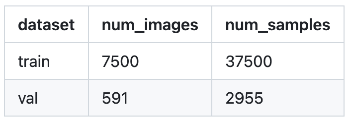
Example from the training set:
{
    'caption': 'A lady is sitting at a table alone in a very colorful place .',
    'img_path': '<your data dir>/flickr8k/Images/3251088971_f4471048e3.jpg'
}
Before training, we need to set up the training code base following the instructions.
The official code requires a zero-shot evaluation on the ImageNet validation set, which is considerably large. For demonstration purposes, we are using the Mini-ImageNet from Kaggle.
The essential training aspects begin with the main function housed in training/main.py.
3.3.1. Data Loaders
A data batch consists of a batch of processed images and texts.
def __getitem__(self, idx):
    images = self.transforms(Image.open(str(self.images[idx])))
    texts = self.tokenize([str(self.captions[idx])])[0]
    # images.shape: [batch_size, 3, 224, 224]
    # texts.shape: [batch_size, 77]
    return images, texts
3.3.1.1. Image Preprocess
Given that the pre-training dataset is sufficiently large, the risk of over-fitting is minimal. As such, the only data augmentation performed during training is a random square crop from resized images.
-
Training preprocess:
Compose( RandomResizedCrop(size=(224, 224), scale=(0.9, 1.0), ratio=(0.75, 1.3333), interpolation=bicubic, antialias=warn) <function _convert_to_rgb at 0x7f0c29104a60> ToTensor() Normalize(mean=(0.48145466, 0.4578275, 0.40821073), std=(0.26862954, 0.26130258, 0.27577711)) ) -
Validation preprocess:
Compose(
    Resize(size=224, interpolation=bicubic, max_size=None, antialias=warn)
    CenterCrop(size=(224, 224))
    <function _convert_to_rgb at 0x7f0c29104a60>
    ToTensor()
    Normalize(mean=(0.48145466, 0.4578275, 0.40821073), std=(0.26862954, 0.26130258, 0.27577711))
)
3.3.1.2. Text Preprocess
The text is tokenized using a lower-cased byte pair encoding (BPE) mechanism, represented within a vocabulary space of 49,152 entries.
- Maximum sequence length: 76
- Each sequence of text begins with a Start of Sentence
[SOS]token (assigned index49406) and concludes with an End of Sentence[EOS]token (index49407).
To illustrate this preprocessing, consider two hypothetical samples from the training set:
batch[1][0] =
tensor([49406,   320,  1929,   536,   518,  2117, 11476,  1095,   518,  1573,
          267,   593,   320,  2172, 14814,   530,   518,  5994,   269, 49407,
            0,     0,     0,     0,     0,     0,     0,     0,     0,     0,
            0,     0,     0,     0,     0,     0,     0,     0,     0,     0,
            0,     0,     0,     0,     0,     0,     0,     0,     0,     0,
            0,     0,     0,     0,     0,     0,     0,     0,     0,     0,
            0,     0,     0,     0,     0,     0,     0,     0,     0,     0,
            0,     0,     0,     0,     0,     0,     0])

batch[1][1] =
tensor([49406,   786,  2862,   525,   518,  5461,   539,  6135,  2252,   550,
         4918,   269, 49407,     0,     0,     0,     0,     0,     0,     0,
            0,     0,     0,     0,     0,     0,     0,     0,     0,     0,
            0,     0,     0,     0,     0,     0,     0,     0,     0,     0,
            0,     0,     0,     0,     0,     0,     0,     0,     0,     0,
            0,     0,     0,     0,     0,     0,     0,     0,     0,     0,
            0,     0,     0,     0,     0,     0,     0,     0,     0,     0,
            0,     0,     0,     0,     0,     0,     0])
3.3.2. Encoders
3.3.2.1. Visual Encoder
The image encoder is trained from scratch without initializing with ImageNet weights. It encodes an image into a 1024-dimensional feature vector.
image_features = self.encode_image(image, normalize=True) if image is not None else None
# image_features: [batch_size, 3, 224, 224] -> [batch_size, 1024], normalized
3.3.2.2. Text Encoder
The text encoder is trained from scratch, and no pre-trained weights are used for initialization. It encodes a text sequence into a 1024-dimensional feature vector.
text_features = self.encode_text(text, normalize=True) if text is not None else None
# text_features: [batch_size, 77] -> [batch_size, 1024], normalized
3.3.3. Training Loop
model_out = model(images, texts)

class CLIP(nn.Module):
    def forward(
        self,
        image: Optional[torch.Tensor] = None,
        text: Optional[torch.Tensor] = None,
    ):
        image_features = (
            self.encode_image(image, normalize=True) if image is not None else None
        )
        text_features = (
            self.encode_text(text, normalize=True) if text is not None else None
        )
        return image_features, text_features, self.logit_scale.exp()

losses = loss(**model_out, output_dict=True)

class ClipLoss(nn.Module):
    def forward(self, image_features, text_features, logit_scale, output_dict=False):
        device = image_features.device
        logits_per_image, logits_per_text = self.get_logits(
            image_features, text_features, logit_scale
        )
        # logits_per_image = logit_scale * image_features @ text_features.T
        # logits_per_text = logit_scale * text_features @ image_features.T

        labels = self.get_ground_truth(device, logits_per_image.shape[0])
        # labels: range(0, batch_size)

        total_loss = (
            F.cross_entropy(logits_per_image, labels)
            + F.cross_entropy(logits_per_text, labels)
        ) / 2

        return {"contrastive_loss": total_loss} if output_dict else total_loss
4. Experiments
4.1. Zero-Shot Transfer
Studying zero-shot transfer is motivated as a method to measure the task-learning capabilities of machine learning systems. From this perspective, a dataset assesses a model’s performance on a task over a specific distribution. This approach is inspired by research in the field of NLP that identifies task learning as an “unexpected side-effect”.
However, this approach faces challenges as many computer vision datasets, initially designed to advance generic image classification, do not necessarily align with measuring performance on specific tasks. While datasets like SVHN can be tied to real-world tasks such as transcribing street numbers from Google Street View photos, the purpose of datasets like CIFAR-10 in evaluating “real” tasks remains ambiguous.
4.1.1. CLIP for Zero-Shot Transfer
CLIP is pre-trained to identify matching pairs of images and text snippets. For zero-shot classification, it uses class names from a dataset as potential text pairings, predicting the most likely image-text pair.
The best CLIP model’s accuracy on ImageNet equals that of the original ResNet-50, even without using its 1.28 million training examples. This equivalence in a zero-shot setting indicates that CLIP is a substantial advance towards versatile and effective zero-shot computer vision classifiers.
4.1.2. Promt Engineering and Ensembling to Improve Zero-Shot Performance
Standard image classification datasets often lack descriptive class information for natural language-based zero-shot transfer, typically using numeric label IDs with separate English name mappings. Some datasets, like Flowers102 and GTSRB, even omit these mappings, hindering zero-shot transfer.
Besides, many datasets’ label choices seem arbitrary, not fitting the needs of successful zero-shot transfer, which relies on precise task descriptions.
Polysemy presents a challenge for CLIP’s text encoder, especially when it receives only class names without context. For example:
- ImageNet includes both birds and machines under “crane”.
- Oxford-IIIT Pet dataset’s “boxer” could mean the dog breed or an athlete.
Distribution mismatch is another issue. CLIP’s pre-training often pairs images with full sentences, not single words.
To tackle these issues, prompt engineering is employed, enhancing the model’s ability to interpret and categorize images more accurately in a zero-shot manner.
Using the prompt template "A photo of a {label}." improves understanding that the text refers to the image, boosting performance (e.g., a 1.3% increase in ImageNet accuracy).
Customizing prompts significantly enhances zero-shot performance, similar to “prompt engineering” with GPT-3. Context-specific category descriptions in prompts lead to improvements, such as:
-
"A photo of a {label}, a type of pet."for Oxford-IIIT Pets,"a type of food"for Food101, and"a type of aircraft"for FGVC Aircraft. - Quotation marks for OCR datasets.
- Clarifying satellite imagery with prompts like
"a satellite photo of a {label}."
In addition to one single prompt, CLIP’s zero-shot performance can be further improved by ensembling multiple zero-shot classifiers, each generated with varied context prompts. These prompts include variations such as "A photo of a big {label}" and "A photo of a small {label}". Here are five sample prompt templates (from a total of 80) that were used specifically for ImageNet:
OPENAI_IMAGENET_TEMPLATES = (
    lambda c: f'a bad photo of a {c}.',
    lambda c: f'a photo of many {c}.',
    lambda c: f'a sculpture of a {c}.',
    lambda c: f'a photo of the hard to see {c}.',
    lambda c: f'a low resolution photo of the {c}.',
)
The ensemble is created using the embedding space rather than the probability space, which allows for the storage of a single set of averaged text embeddings, ensuring that the computational cost of the ensemble remains equivalent to using a single classifier when distributed over numerous predictions.
4.1.3. Analysis of Zero-Shot CLIP Performance
4.1.3.1. Zero-Shot CLIP VS. Fully Supervised Models
CLIP is competitive with a fully supervised baseline. Across a 27 dataset eval suite, a zero-shot CLIP classifier outperforms a fully supervised linear classifier fitted on ResNet-50 features on 16 datasets, including ImageNet.
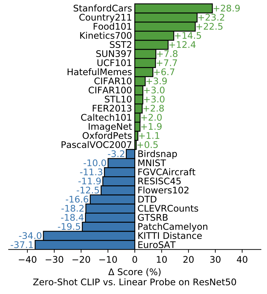 Image source: original paper Figure 5
Looking at CLIP’s performance on different types of datasets reveals some interesting behavior.
- Inconsistent: fine-grained classification (Stanford Cars, Food101, Flowers102, FGVCAircraft, OxfordPets, Birdsnap), potentially due to varying amounts of per-task supervision between WIT and ImageNet.
- Similar: general object classification (ImageNet, CIFAR10/100, STL10, PascalVOC2007).
- Strong: action recognition in videos (Kinetics700, UCF101), potentially due to natural language providing wider supervision for visual concepts involving verbs, compared to the noun-centric object supervision in ImageNet.
- Weak: specialized, complex, or abstract tasks, such as satellite image classification, lymph node tumor detection, counting objects in synthetic scenes, and self-driving related tasks such as german traffic sign recognition, recognizing distance to the nearest car.
CLIP’s zero-shot performance has a strong positive correlation (0.82) to linear probe performance, though it is generally 10 to 25 points lower.
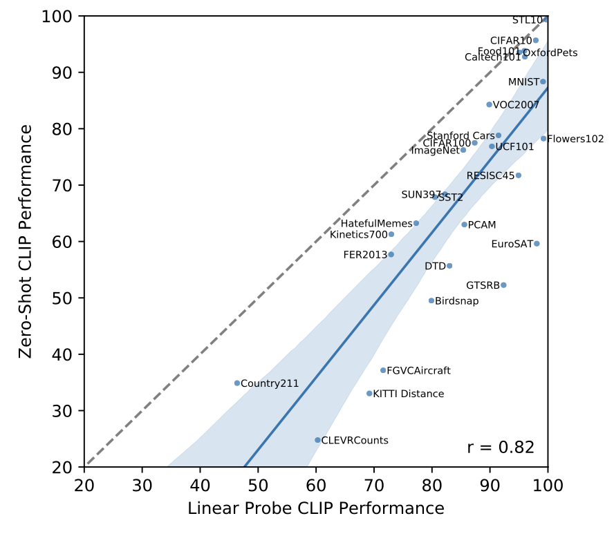 Image source: original paper Figure 8
It comes close on five datasets (STL10, CIFAR10, Food101, OxfordPets, and Caltech101), where both zero-shot and fully supervised accuracies exceed 90%. This implies that CLIP is likely more adept at zero-shot transfer when its internal representations are of high quality.
4.1.3.2. Zero-Shot CLIP VS. Few-Shot Models
Zero-shot CLIP outperforms few-shot linear probes and nearly matches the best results of a 16-shot linear classifier across publicly available models.
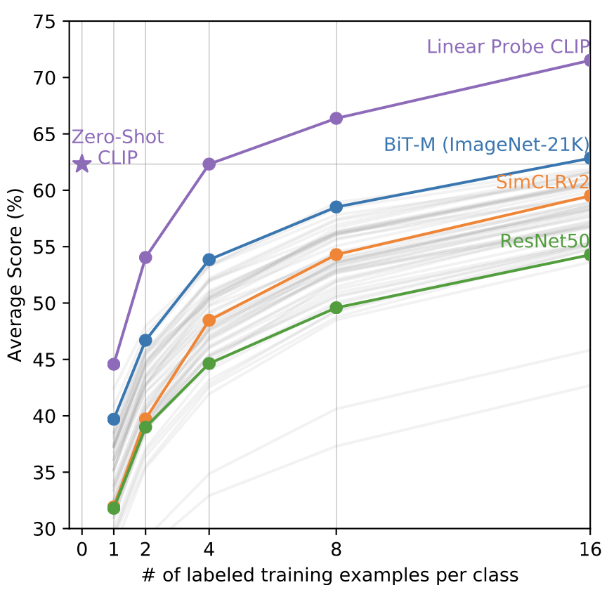 Image source: original paper Figure 6
The result is contrary to expectations that zero-shot performance would lag behind few-shot, zero-shot CLIP actually matches the performance of 4-shot logistic regression in the same feature space. This is likely due to an important difference between the zero-shot and few-shot approach.
Zero-shot CLIP generates its classifier through natural language, enabling direct specification of visual concepts. In contrast, traditional supervised learning methods must deduce concepts indirectly from training examples.
The downside of example-based learning without context is that numerous hypotheses can align with the data, particularly in one-shot scenarios. A single image can depict numerous visual concepts, and while an adept learner might leverage visual cues and heuristics (such as assuming the main object in an image represents the concept), there are no guarantees.
An attempt is made to estimate the number of labeled examples per class would be required for a logistic regression classifier, using the same feature space, to match the performance of zero-shot CLIP on various datasets.
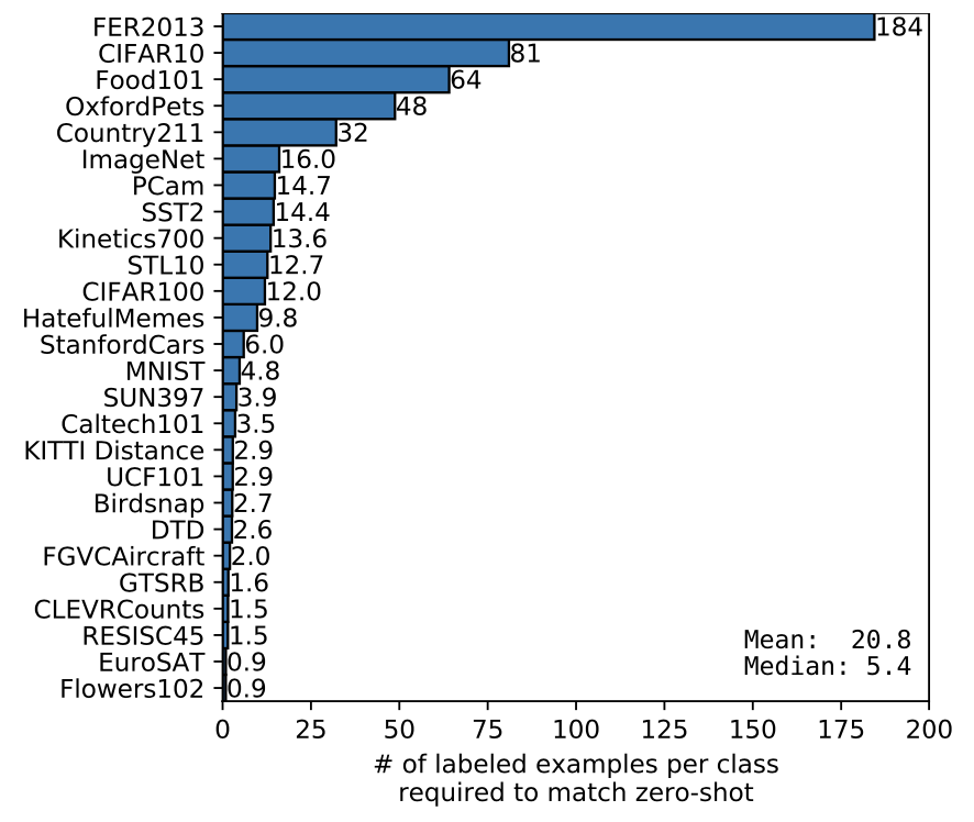 Image source: original paper Figure 7
It is found that zero-shot transfer can have widely varying efficiency across datasets, ranging from less than one labeled example per class to 184.
4.2. Representation Learning
The capabilities of CLIP in learning representations are investigated by training a linear classifier on the model-derived representations, followed by evaluating its performance across various datasets.
While small CLIP models such as a ResNet-50 and ResNet-101 outperform other ResNets trained on ImageNet-1K (BiT-S and the originals), they underperform ResNets trained on ImageNet-21K (BiT-M). These small CLIP models also underperform models in the EfficientNet family with similar compute requirements.
However, models trained with CLIP scale very well and the largest model (ResNet-50x64) slightly outperforms the best performing existing model (a Noisy Student EfficientNet-L2) on both overall score and compute efficiency.
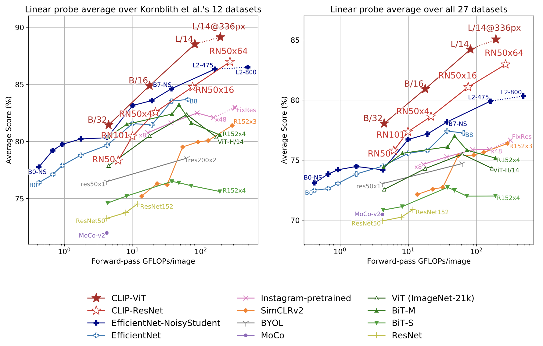 Image source: original paper Figure 10
It is also found that CLIP vision transformers demonstrate approximately 3 times the compute efficiency compared to CLIP ResNets, enabling the achievement of higher overall performance within the given compute budget.
CLIP models showcase a remarkable ability to learn a diverse array of tasks from scratch, including geo-localization, optical character recognition, facial emotion recognition, and action recognition.
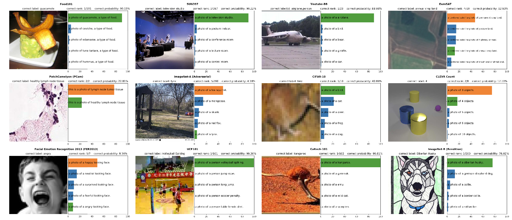 Image source: original paper Figure 21
However, this range is not fully captured in the 12-dataset evaluation suite, which leans towards ImageNet-related tasks. To address this, CLIP is evaluated on a more extensive 27-dataset evaluation suite that incorporates a variety of tasks such as German Traffic Sign Recognition and other datasets adapted from VTAB. In this broader scope, the advantages of CLIP become more evident.
This broader evaluation also reveals stronger performance from self-supervised systems. For instance, whereas SimCLRv2 is outpaced by BiT-M in the 12-dataset evaluation suite, it surpasses BiT-M in the 27-dataset suite.
These results underline the importance of expanding task diversity for a comprehensive understanding of a system’s “general” capabilities.
CLIP surpasses the Noisy Student EfficientNet-L2 on 21 out of the 27 datasets, showing notable improvements in OCR tasks (SST2 and HatefulMemes), geo-localization and scene recognition (Country211, SUN397), as well as activity recognition in videos (Kinetics700 and UCF101). It also excels in fine-grained car and traffic sign recognition (Stanford Cars and GTSRB).
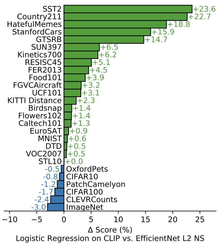 Image source: original paper Figure 11
However, it still underperforms the EfficientNet on several datasets. Unsurprisingly, the dataset that the EfficientNet does best relative to CLIP on is the one it was trained on: ImageNet.
The EffcientNet also slightly outperforms CLIP on low-resolution datasets such as CIFAR10 and CIFAR100, potentially due to CLIP’s lack of scale-based data augmentation. Furthermore, on PatchCamelyon and CLEVRCounts, where both models show relatively low performance, EfficientNet performs slightly better.
4.3. Robustness to Natural Distribution Shift
Taori et al. study how the performance of ImageNet models change when evaluated on natural distribution shifts, measuring performance on a set of 7 distribution shifts:
- ImageNetV2
- ImageNet Sketch
- Youtube-BB
- ImageNet-Vid
- ObjectNet
- ImageNet Adversarial
- ImageNet Rendition
They differentiate these datasets, comprised of novel images collected from a variety of sources, from synthetic distribution shifts like ImageNet-C, Stylized ImageNet, and adversarial attacks, which involve manipulated existing images.
This distinction is crucial as many methods enhancing performance on synthetic shifts do not consistently translate to improvements on natural distributions.
Zero-shot CLIP is much more robust to distribution shift than standard ImageNet models.
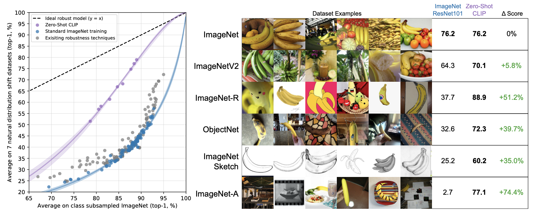 Image source: original paper Figure 13
However, while these results show that zero-shot models can be much more robust, they do not necessarily mean that supervised learning on ImageNet causes a robustness gap. Other details of CLIP, such as its large and diverse pre-training dataset or use of natural language supervision could also result in much more robust models regardless of whether they are zero-shot or fine-tuned.
Therefore, the change in performance of CLIP models from the zero-shot classifier is also measured after adapting to the ImageNet distribution through an L2 regularized logistic regression classifier fitted to CLIP features on the ImageNet training set.
While supervised adaptation to ImageNet raises ImageNet accuracy by 9.2%, it results in a slight decrease in average robustness.
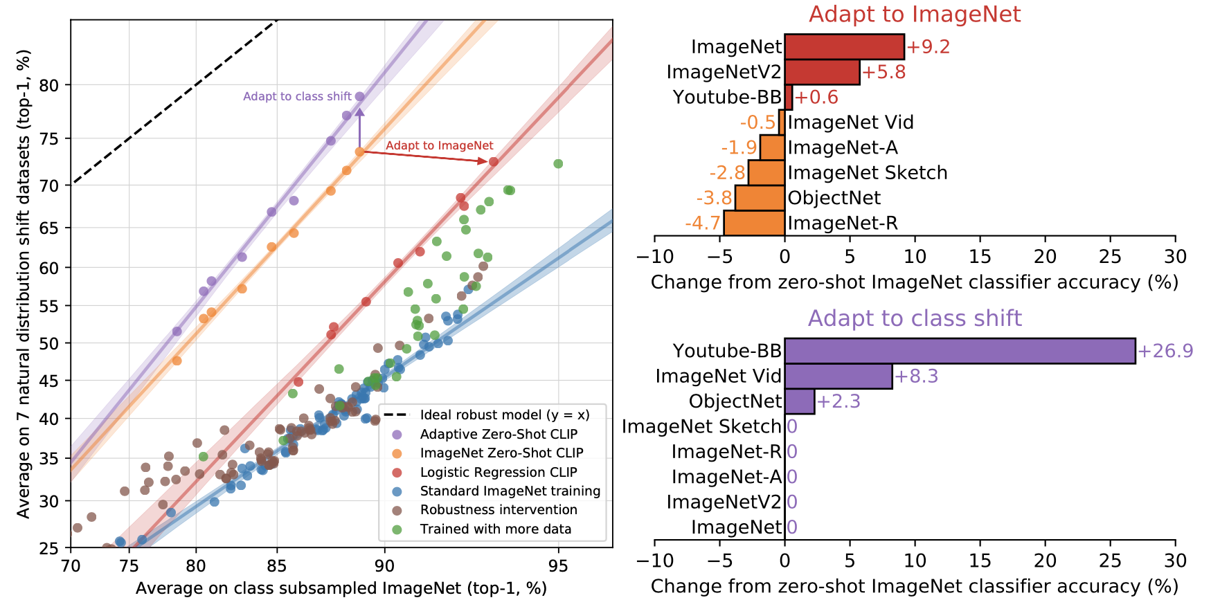 Image source: original paper Figure 14
Another robustness intervention is also investigated, enabling by flexible zero-shot natural-language-based image classifiers. The target classes across the 7 transfer datasets are not always perfectly aligned with those of ImageNet. Two datasets, Youtube-BB and ImageNet-Vid, consist of super-classes of ImageNet. This presents a problem when trying to use the fixed 1000-way classifier of an ImageNet model to make predictions.
Taori et al. addressed this by max-pooling predictions across all sub-classes based on the ImageNet class hierarchy. However, this approach sometimes provides an imperfect mapping. For instance, for the “person” class in Youtube-BB, predictions are pooled over various unrelated ImageNet classes, such as a baseball player, a bridegroom, and a scuba diver. In contrast, with CLIP, a custom zero-shot classifier can be generated for each dataset directly using its own class names.
This approach is observed to improve average effective robustness by 5%, although the improvements are significantly concentrated on just a few datasets. Interestingly, accuracy on ObjectNet also sees a boost of 2.3%. Despite ObjectNet being designed to closely correspond with ImageNet classes, utilizing the class names provided by the creators of ObjectNet still offers a marginal benefit over using ImageNet class names and resorting to prediction pooling when necessary.
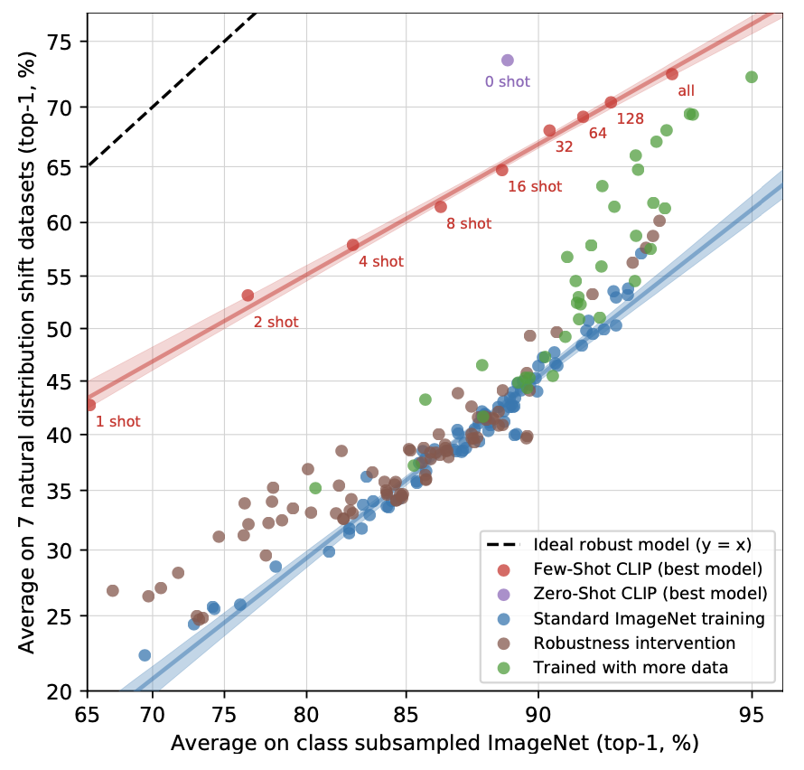 Image source: original paper Figure 15
The visualization shows the performance of 0-shot, 1-shot, 2-shot, 4-shot …, 128-shot, and fully supervised logistic regression classifiers on the best CLIP model’s features. Few-shot CLIP also increases effective robustness compared to existing ImageNet models but is less robust than zero-shot CLIP.
5. Comparison to Human Performance
The study sought to understand the level of human zero-shot performance on these evaluation tasks and the extent to which human performance is enhanced when individuals are shown one or two image samples.
Notably, human participants’ average performance increased from 54% to 76% with the introduction of just one training example per class. Moreover, the incremental benefit of providing a second training example was found to be minimal.
The gain in accuracy going from zero to one shot is almost entirely on images that humans were uncertain about. This suggests that humans “know what they don’t know” and are able to update their priors on the images they are most uncertain in based on a single example.
The observations indicate a significant disparity between human learning from limited examples and the few-shot learning methods utilized in the study. The few-shot evaluations of CLIP may not fully leverage prior knowledge, unlike human learners. Consequently, integrating prior knowledge into few-shot learning could represent a crucial advancement in refining the algorithms underlying CLIP.
Furthermore, the hardest problems for CLIP also tend to be the hardest problems for humans., potentially due to at least a two factors: noise in the dataset (including mislabeled images) and out of distribution images being hard for both humans and models.
6. Data Overlap Analysis
The issue of unintended data overlap between large pre-training datasets from the internet and evaluation datasets was examined. This overlap could potentially compromise the evaluations’ ability to accurately measure the model’s generalization.
With a median overlap of 2.2% and an average of 3.2%, the influence on overall accuracy was minor for most datasets, suggesting that the overlap did not significantly boost model performance.
An interesting point is the possible change in data distribution between the Overlap and Clean subsets. For example, in Kinetics-700, many “overlaps” were just all-black transition frames, leading to a 20% accuracy drop in the Overlap subset.
This indicates more subtle distribution shifts, implying accuracy changes might be due to class distribution changes or the difficulty of duplicates, rather than over-fitting. However, these shifts could mask the true level of over-fitting.
7. Limitations
-
It’s estimated that around 1000x increase in computational power is needed for zero-shot CLIP to achieve state-of-the-art performance, which is currently unattainable with existing hardware. Enhancing computational and data efficiency is crucial.
-
CLIP’s zero-shot performance is still quite weak on several kinds of tasks, especially the noval tasks which are unlikely to be included in CLIP’s pre-training dataset.
-
CLIP demonstrates poor generalization to truly out-of-distribution data, as evidenced by its 88% accuracy on handwritten MNIST digits. This suggests CLIP does little to address the underlying problem of brittle generalization of deep learning models. Instead CLIP tries to circumvent the problem and hopes that by training on such a large and varied dataset that all data will be effectively in-distribution.
-
CLIP is constrained to selecting from predefined concepts in zero-shot classifiers, lacking the generative flexibility of approaches like image captioning that can produce novel outputs.
-
Developing a benchmark specifically for evaluating broad zero-shot transfer capabilities is essential, moving away from the reuse of existing supervised datasets.
-
Training on unfiltered internet data causes CLIP models to inherit and perpetuate social biases, highlighting the necessity for careful data curation and bias mitigation strategies.
-
Many complex tasks and visual concepts can be difficult to specify just through text. Actual training examples are undeniably useful but CLIP does not optimize for few-shot performance directly. Future work is needed to develop methods that combine CLIP’s strong zero-shot performance with efficient few-shot learning.
Afterwords: Thoughts on CLIP
It’s been a great time reading the CLIP paper, as it provides a comprehensive evaluation of the CLIP model along with valuable insights.
In this session, I share my personal reflections regarding CLIP. Ultimately, I believe that one’s own insights are the most precious outcomes of immersing oneself in the great accomplishments of others.
Natural language acts as a direct medium for conveying our intentions to the machine learning model
Projecting different modalities into a unified space, as done by CLIP, brings machine learning systems closer to human-like understanding. CLIP’s combination of visual concepts with natural language fosters direct communication with machine learning models, enhancing tasks like zero-shot classification.
Traditional machine learning lacks a direct method for models to understand the intent behind tasks or the meanings of class names. Models learn from examples, focusing on grouping similar patterns without comprehending their significance. This lack of understanding limits the effectiveness of few-shot and one-shot learning, as models can’t discern multiple concepts in a single image, necessitating extensive data to properly learn classifications.
For example, distinguishing turtles from tortoises requires varied images to teach the model relevant classification details, instead of associating species with their backgrounds. Without understanding class names, models might classify based on irrelevant factors like sea or land backgrounds.
This approach leads to a lack of transparency in how models understand concepts, potentially misaligning with human intentions and risking ineffective performance. In contrast, integrating visual concepts with natural language provides a more explicit and effective way to convey objectives, mirroring human communication. However, success in this method hinges on humans clearly understanding and articulating their intentions in natural language.
Example-based learning remains valuable, as not all concepts are expressible through natural language
Natural language has limitations, as CLIP struggles with specialized or abstract tasks like satellite image classification, tumor detection, object counting in synthetic scenes, and autonomous driving-related tasks. This may be due to scarce relevant data in its pre-training set and the challenge of expressing certain concepts in natural language, like associating visual cues with abstract measurements.
For such complex tasks, example-based learning remains practical when experts can provide visual ground truth. However, for some tasks, combining multiple modalities might be necessary.
The CLIP training process encompasses its own implicit perspectives
Example-based learning, as previously discussed, is implicit, with objectives inferred from examples and specific patterns recognized by the model often unclear. CLIP, while linking natural language with visual concepts, also has implicit elements.
The image encoder condenses an entire image into a single vector, hiding which visual concepts are represented. With limited capacity, it may omit less important concepts, leaving us in the dark about what’s excluded. The text encoder similarly reduces sentences to a single vector, making it uncertain which words or phrases are emphasized or ignored.
The richness of the original images or text heavily influences these vectors’ completeness. This is akin to example-based learning, where the patterns the model recognizes and their alignment with human intentions are not transparent. The exact contents of CLIP’s vectors remain elusive.
Thus, the size and diversity of the pre-training dataset and the model’s capacity are crucial. A larger, more varied dataset enables the model to recognize and encode a broader range of concepts. A more substantial model can encode finer details in its representations.
Transformers seem to work better together
The paper highlights that the ViT-L/14@336px model yields the best performance. While the ViT paper had already demonstrated the superior capabilities of visual transformers over convolutional networks, this leads to a fascinating inquiry: Does the pairing of two transformers - one for images and another for text - result in an inherently more harmonious integration than combining a convolutional network with a text transformer?
The image encoding task might be harder than the text encoding task
The paper discloses that variations in the capacity of the text encoder do not substantially impact CLIP’s performance. This suggests that the task of text encoding in CLIP might be more straightforward.
Conversely, the extraction of visual concepts from images seems to be a more complex challenge. Unlike sentences, which can be organically broken down into words and phrases, segmenting an image into discrete concepts is not as intuitive.
A comprehensive evaluation suite specifically designed to assess the general task learning capabilities is lacking
The authors have made efforts to compile a diverse collection of 27 datasets for evaluation. Nonetheless, these datasets are adaptations of pre-existing ones and may not have been designed with enough precision to measure a model’s task-specific performance accurately.
For example, the test sets might not be comprehensive, missing key aspects of the intended task, which could result in selection bias during evaluation. Therefore, creating a more sophisticated and tailored evaluation suite is essential for the progression of the field and for more precise assessments of foundational models’ capabilities.
Combine the strengths of zero-shot transfer with the adaptability of few-shot learning
Humans significantly boost their few-shot learning performance, going from 54% to 76% accuracy with just one example per class, while the zero-shot CLIP model matches the 4-shot logistic regression using identical features.
The critical difference is humans’ understanding of the task’s goals and their ability to seek clarification. In zero-shot tasks, they recognize their knowledge gaps and use extra examples to improve accuracy.
However, CLIP’s performance in few-shot scenarios doesn’t increase as expected. Unlike humans, the model doesn’t seem to effectively use additional examples to enhance learning, suggesting a loss of prior knowledge or a difficulty in assimilating new information.
The example-based learning method has inherent limitations
In tasks requiring human-level few-shot learning, performance often plateaus after seeing more than one example per class, indicating that simply providing more examples may not be enough for significant improvement. Humans might need additional information or guidance, especially if their existing assumptions about the task are incorrect.
For example, if people have mistaken ideas about what distinguishes classes, they might approach the task incorrectly with confidence. Correcting this could require either explicit expert guidance or access to a much larger set of examples to learn the correct criteria, which is more challenging than following expert advice.
This raises intriguing questions about the roles of guidance, pre-existing knowledge, and example-based learning in human understanding, highlighting areas where human learning could benefit from better instruction and clarification.
CLIP is powerful, but not omniscient and omnipotent
CLIP’s ability to learn a wide range of concepts through representation learning is expected, given its training on a dataset larger and more diverse than ImageNet or Instagram, encompassing various internet-based concepts.
However, CLIP’s learning is limited to its internet-based data source. Since the internet covers only part of human knowledge and lacks non-digitized or incomplete information, CLIP’s understanding is similarly restricted. It can’t comprehend what’s not available online.
This highlights the ongoing need for specialized models tailored for specific tasks, to fill in CLIP’s knowledge gaps and address the subtleties of diverse real-world applications.
CLIP’s robustness is largely attributed to its diverse training dataset
CLIP’s pre-training dataset from the internet is diverse in form, style, and photographic conditions. However, it’s important to note that CLIP struggles with truly out-of-distribution examples, like the handwritten digits in the MNIST dataset.
This situation is akin to human learning patterns, such as studying for multiple exams. Having a broad knowledge base but focusing too much on one subject can unintentionally harm performance in others. This comparison highlights CLIP’s limitations and parallels human learning, suggesting areas for improvement in machine learning models.
Reference
- Paper: Learning Transferable Visual Models From Natural Language Supervision
- Code: https://github.com/mlfoundations/open_clip
- Cover image source: https://openai.com/research/clip
